Contents

Analysis Operator

The analysis operator W is p -by- n iid Gaussian and thus a nearly uniform and nearly tight frame

n=1e3; % signal dimension
overcompleteness = 2.0; % ratio of analysis dimension to signal dimension
p=round(n*overcompleteness); % analysis dimension
W = randn(p,n) / sqrt(n); % analysis operator with approximately unit-norm rows

Measurement Matrix

The measurement operator M is m -by- n iid Gaussian

delta = 0.5 + (overcompleteness-1)*0.25; % sampling ratio
m=round(delta*n); % number of measurements
M = randn(m,n)/sqrt(n);  % measurement operator with approximately unit-norm rows

Cosparse Signal

The signal x is l-cosparse on W, i.e., W * x has l zeros, located uniformly at random

rho = .3;  % rho=(n-l)/m: an uncertainty parameter between 0 (easy) and 1 (difficult)
l=n - round(rho*m);  % cosparsity: the number of zeros in W*x
cosup = randperm(p,l); % cosupport: a random selection of l rows
P = null(W(cosup,:)); % the rows of P form a basis for the nullspace of the cosupported rows of W
x = P*P'*randn(n,1); % a random cosparse signal created by projecting onto the nullspace
x = x/norm(x);
z = M*x; % true noiseless measurements
v = W*x; % true analysis outputs

Noisy Compressive Linear Measurements

The measurements are constructed as y = M x + w with AWGN w

SNRdB = 80; % measurement signal-to-noise ratio in dB
wvar = (norm(z)^2/m) * 10^(-SNRdB/10); % AWGN variance
y = z + randn(m,1)*sqrt(wvar); % noisy measurements

Configuring and Running GrAMPA

GrAMPA is based on the generalized approximate message passing (GAMP) algorithm, a powerful Bayesian framework for large-scale generalized-linear inference exploiting a separable signal prior, a separable likelihood, and a sufficiently large, dense, linear transform.

To get started using GAMP, download the latest GAMPmatlab release. You can find some introductory examples described on the wikia site as well as intructions on how to get the latest development code.

The workhorse of GAMPmatlab is the gampEst function. To implement GrAMPA, we need to specify its four input arguments: the signal prior GrampaEstimIn, the measurement likelihood GrampaEstimOut, the linear transform GrampaLinTrans, and the algorithmic options GrampaOptions.

% When using GAMP to implement GrAMPA, we recommend the following options.
GrampaOptions = GampOpt('legacyOut',false,'uniformVariance',true,'adaptStep',false);
GrampaOptions.xvar0 = (norm(y)^2-wvar*m)/norm(M,'fro')^2; % guess at signal variance
GrampaOptions.step = 0.1; % initial stepsize
GrampaOptions.stepMax = 0.5; % maximum stepsize
GrampaOptions.stepIncr = 1.01; % stepsize increase rate
GrampaOptions.tol = 1e-6; % stopping tolerance
GrampaOptions.nit = 1000; % maximum number of iterations
GrampaOptions.varNorm = true; % turn on internal normalization
GrampaOptions.zvarToPvarMax = inf; % analysis variance clipping ratio

% For this example, we assume nothing about the signal, and so we use the trivial
% signal prior.  If we knew the signal was bounded on an interval, we would
% instead use *UnifEstimIn*
GrampaEstimIn = NullEstimIn(0,1);

% GrampaLinTrans is constructed by "stacking" the measurement operator
% on top of the analysis operator.  Since our operators are explicit matrices,
% we can simply stack the matrices, but in general we'd use *LinTransConcat()*.
% Note that, when stacking, the operators must have the same (average) row norms,
% which in this example is ensured by the way that we built the operators.
GrampaLinTrans = [M;W];
iMeas = (1:m)';	% measurement output indices
iAnal = (1:p)'+m; % analysis output indices

% The likelihood is then constructed by stacking the measurement likelihood
% on top of the analysis prior.  In this example, the measurement likelihood is AWGN
% with variance *wvar*.  For the analysis prior, we use ``SNIPEstim,'' which depends on
% a parameter *omega*.  Below, we guess the value *omega*=3.
MeasEstimOut = AwgnEstimOut(y,wvar);
omega = 3;
AnaEstimOut = SNIPEstim(omega);
GrampaEstimOut = EstimOutConcat({MeasEstimOut;AnaEstimOut},[m,p]);

% Finally, we call *gampEst* using the objects contructed above, and measure the
% resulting normalized output SNR.
estFin1 = gampEst(GrampaEstimIn,GrampaEstimOut,GrampaLinTrans,GrampaOptions);
snr_gamp1 = 20*log10( norm(x)/norm(x-estFin1.xhat) );
fprintf('With guessed omega=%.1f, GrAMPA gives NMSE=%.2fdB\n',AnaEstimOut.omega,-snr_gamp1);

With guessed omega=3.0, GrAMPA gives NMSE=-81.87dB

An Oracle Bound

The "cosupport genie" magically knows the true cosupport and then finds the signal vector that best matches the measurements (in a least-squares sense) while yielding that cosupport. To implement this, we can use the previously constructed matrix P, whose rows must now be orthogonal to the genie estimate of x:

xhat_genie = P * ( [M*P] \ y ); % solve LLS over that subspace
gMSEx = norm(x-xhat_genie)^2;
snr_genie = 10*log10( norm(x)^2/gMSEx );
fprintf('Meanwhile, the cosupport genie gives NMSE=%.2fdB\n',-snr_genie)

Meanwhile, the cosupport genie gives NMSE=-83.26dB

SURE Tuning of SNIPEstim:

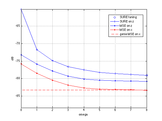
Now let's see if we can improve performance by (genie) tuning the SNIPEstim parameter omega using Stein's Unbiased Risk Estimate (SURE) computed from the GAMP analysis outputs, which should be AWGN corrupted versions of true analysis outputs with known noise variance. We will also compute the true signal MSE to verify that SURE is working as expected.

% First, let's compute the SURE estimates over a grid of omegas
fprintf('Tuning *omega* by computing SURE risk over a grid...\n')
omegaGrid = linspace(0,8,9)'; % typical range for SNIPEstim *omega*
SURE = zeros(size(omegaGrid));
MSEx = zeros(size(omegaGrid));
for i=1:length(omegaGrid)
    % run GrAMPA at an omega on the grid
    AnaEstimOut = SNIPEstim(omegaGrid(i));
    GrampaEstimOut = EstimOutConcat({MeasEstimOut;AnaEstimOut},[m,p]);
    estFin2 = gampEst(GrampaEstimIn, GrampaEstimOut, GrampaLinTrans, GrampaOptions);
    phat = estFin2.phat;
    pvar = estFin2.pvar;
    zhat = estFin2.zhat;
    zvar = estFin2.zvar;

    % compute SURE approximation to analysis-coefficient MSE at hypothesized omega
    SURE(i) = sum(abs(-pvar + abs(zhat - phat).^2 + 2*zvar));

    % compute true signal-MSE at hypothesized omega (requiring knowledge of signal)
    xhat = estFin2.xhat;
    MSEx(i) = norm(xhat - x)^2;
    MSEz(i) = norm(zhat - [z;v])^2;
end
[bestSURE,iBest] = min(SURE);
bestOmega = omegaGrid(iBest);
snr_gamp2 = 10*log10( norm(x)^2/MSEx(iBest) );
disp('')
fprintf('With SURE-tuned omega=%.1f, GrAMPA gives NMSE=%.2fdB\n',bestOmega,-snr_gamp2);

% Finally, let's plot GrAMPA's MSE versus *omega* along with the SURE-estimated risk
figure(1); clf;
  plot(bestOmega,10*log10(bestSURE),'bo',...
       omegaGrid,10*log10(SURE),'b+-',...
       omegaGrid,10*log10(MSEz),'b.-',...
       omegaGrid,10*log10(MSEx),'r.-',...
       omegaGrid,10*log10(gMSEx)*ones(size(omegaGrid)),'r--');
  axe1=axis; axis('tight'); axe2=axis; axis([axe1(1:2),axe2(3)-5,min(axe2(4),axe2(3)+50)])
  grid on;
  legend('SURE tuning','SURE on z','MSE on z','MSE on x','genie MSE on x','Location','Best')
  ylabel('dB')
  xlabel('omega')

Tuning *omega* by computing SURE risk over a grid...
With SURE-tuned omega=8.0, GrAMPA gives NMSE=-83.30dB

Published with MATLAB® R2013a