EM-NN-AMP Algorithm: A succinct overview
Jeremy Vila, Oct. 2013
EM-NN-AMP attempts to recover a sparse signal of length N through (possibly) noisy measurements of length M (with perhaps M < N). We model this through the linear system
 .
.
We focus on non-negative (NN) signals that obey the linear equality constraints
 .
.
EM-NN-AMP is comprised of three different algorithms: NN least-squares AMP (NNLS-AMP), expectation maximization NN LASSO AMP (EM-NNL-AMP), and EM NN Gaussian mixture AMP (EM-NNGM-AMP). Toggling between them using the EMNNAMP Matlab code is extremely easy.
Refer to the paper EM-NN-AMP by Jeremy Vila Philip Schniter for a detailed description of the algorithm. This manual will show how to use the EM-NN-AMP MATLAB code.
Contents
Example 1: Non-negative Uniform Data
The following example will use randomly generated data drawn from a uniform distribution
close all
clear all

N = 500; %Fix dimension of signal
M = 1000;  %Fix number of measurements
SNR = 30; %Fix signal to noise ratio

% Form A matrix from i.i.d. Gaussian entries
% Generate normalized random sensing matrix
Amat = randn(M,N);
columnNorms = sqrt(diag(Amat'*Amat));
Amat = Amat*diag(1 ./ columnNorms); %unit norm columns
A = MatrixLinTrans(Amat);

%Generate non-sparse uniform signal
x = rand(N,1);

%Compute true noiseless measurement
ztrue = A.mult(x);

%Output channel- Calculate noise level
muw = norm(ztrue)^2/M*10^(-SNR/10)

%Compute noisy output
y = ztrue + sqrt(muw)*(randn(M,1));
EM-NN-AMP is comprised of the NNLS-AMP, EM-NNL-AMP, and EM-NNGM-AMP algorithms. Toggling between them is straightforward. To run each algorithm on its defaults, all one needs to supply are the measurements and mixing matrix (or operator). The algorithm then returns the recovered linearly-constrained non-negative signal.
time = tic;
optALG.alg_type = 'NNLSAMP'; %Pick the NNLS-AMP algorithm
xhat = EMNNAMP(y, A, optALG); %Perform EMNNAMP
time = toc(time) %Calculate total time
time =

    0.2637
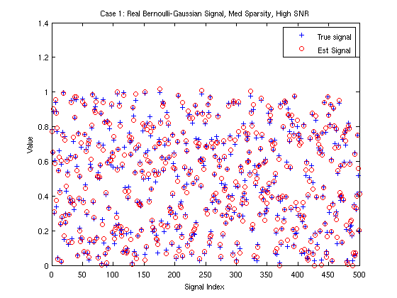
Verify accuracy of signal recovery with NMSE and plots
nmse = 10*log10(norm(x-xhat)^2/norm(x)^2) % Report NNLSAMP's NMSE (in dB)

figure(1)
plot(x,'b+');hold on %Plot true signal
plot(xhat,'ro'); hold off %Plot signal estimates
xlabel('Signal Index'); ylabel('Value')
title('Case 1: Real Bernoulli-Gaussian Signal, Med Sparsity, High SNR')
legend('True signal', 'Est Signal')
nmse =

  -30.1565
It is straightforward to run EM-NNL-AMP and EM-NNGM-AMP using the EMNNAMP Matlab code. Moreover, parameter initialization and learning are handled automatically.
Run EM-NNL-AMP
time = tic;
optALG.alg_type = 'NNLAMP'; %Pick the EM-NNL-AMP algorithm
xhat = EMNNAMP(y, A, optALG); %Perform EMNNAMP
time = toc(time) %Calculate total time
nmse = 10*log10(norm(x-xhat)^2/norm(x)^2) % Report NNLSAMP's NMSE (in dB)
time =

    0.1077


nmse =

  -29.2548
Run EM-NNGM-AMP
time = tic;
optALG.alg_type = 'NNGMAMP'; %Pick the EM-NNGM-AMP algorithm
xhat = EMNNAMP(y, A, optALG); %Perform EMNNAMP
time = toc(time) %Calculate total time
nmse = 10*log10(norm(x-xhat)^2/norm(x)^2) % Report NNLSAMP's NMSE (in dB)
time =

    0.6455


nmse =

  -30.2019
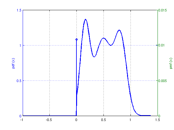
Alternatively, one can call xhat = EMNNAMP(y, A), as EMNNAMP assumes optALG.alg_type = 'NNGMAMP'; as the default
time = tic;
[xhat,stateFin] = EMNNAMP(y, A); %Perform EMNNAMP
time = toc(time) %Calculate total time
nmse = 10*log10(norm(x-xhat)^2/norm(x)^2) % Report NNLSAMP's NMSE (in dB)

% It is straightforward plot the recovered NNGM signal distribution
figure(2)
plot_NNGM(stateFin);
time =

    0.5392


nmse =

  -30.2019
Example 2: Enforcing linear equality constraints
EM-NN-AMP can also handle other signal types including those with linear equality constraints, even in the compressive sensing regime.
clear('optALG'); %clear previous optALG options

N = 500; %Fix dimension of signal
del = 0.5; %undersampling ratio del = M/N
rho = 0.3; %normalized sparsity rate rho = K/M
SNR = 40; %Signal to noise ratio (dB)

M = ceil(del*N); %Find appropriate measurement size
K = floor(rho*M); %Find appropriate sparsity
if K == 0
    K = 1; %Ensure at least one active coefficient.
end

% Form A matrix
%Generate normalized random sensing matrix
Amat = randn(M,N);
columnNorms = sqrt(diag(Amat'*Amat));
Amat = Amat*diag(1 ./ columnNorms); %unit norm columns
A = MatrixLinTrans(Amat);

%Generate signal
x = dirrnd(10*ones(1,K),1)';
x(end+1:N) = zeros(N-K,1);
x = x(randperm(N));

%Compute true noiseless measurement
ztrue = A.mult(x);

%Output channel- Calculate noise level
muw = norm(ztrue)^2/M*10^(-SNR/10);

%Compute noisy output
y = ztrue + sqrt(muw)*(randn(M,1));

time = tic;
optALG.linEqMat = ones(1,N); %supply linear equality matrix B
optALG.linEqMeas = 1; %supply linear equality "measurement" c
xhat = EMNNAMP(y, A, optALG); %Perform EM-NNGM-AMP
time5 = toc(time) %Calculate total time
nmse = 10*log10(norm(x-xhat)^2/norm(x)^2) %Report recovery nmse in dB
LE_nmse = 10*log10(norm(1-sum(xhat))^2) %Report the nmse of linear equality constraint
time5 =

    0.7370


nmse =

  -43.6912


LE_nmse =

  -81.0532
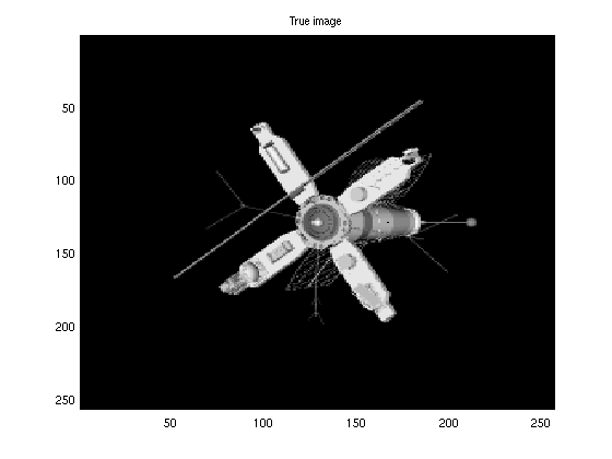
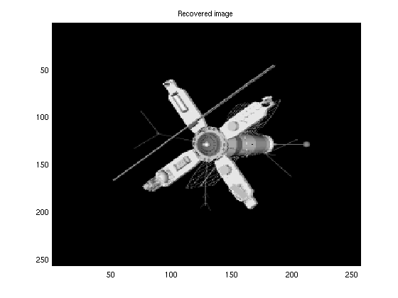
Example 3: Real NN satellite image in compressive sensing regime
It is straightforward to apply EMNNAMP to real NN datasets. In this example, we recover a sparse NN image of a satellite under noisy, compressed linear measurements using the randomly row-sampled Hadamard transform operator.
clear('optEM') %clear previous options

%load image and plot it
load('satimage.mat','x')
figure(3)
imagesc(x);
colormap('gray')
title('True image')

%Find dimension of signal and vectorize it
N = numel(x);
x = reshape(x,N,1);

del = 0.3; %del = M/N
SNR = 60; %Define SNR

%Specify number of measurements
M = ceil(del*N);

%Build ``wide'' fast Walsh-Hadamard transform
A = FWHTLinTrans(N,[],1);
%get indeces of rows randomly
ind = A.ySamplesRandom(M);
%subsample by either method
A.ySamplesSetFromSubScripts(ind);

ztrue = A.mult(x); %Generate measurements

muw = norm(ztrue)^2/M*10^(-SNR/10); %Calculate noise level

y = ztrue + sqrt(muw)*randn(M,1); %Compute noisy output

tstart = tic;
optEM.maxEMiter = 20; %decrease maximum EM iterations
optGAMP.adaptStep = false; %Turn off adaptive step size
optGAMP.verbose= true; %Turn on GAMP verbosity
xhat = EMNNAMP(y, A,[],optEM,optGAMP); %Perform EMNNGMAMP
time = toc(tstart)
nmse = 10*log10(norm(x-xhat)^2/norm(x)^2) % Report EMNNAMP's NMSE (in dB)

%plot the recovered image
figure(4)
xhat = reshape(xhat,sqrt(N),sqrt(N));
imagesc(xhat)
colormap('gray')
title('Recovered image')
it=  1  value=        -Inf  step=1.000000  |dx|/|x|=         NaN
it=  2  value=        -Inf  step=1.000000  |dx|/|x|=  8.9293e-01
it=  3  value=        -Inf  step=1.000000  |dx|/|x|=  4.5428e-01
it=  4  value=        -Inf  step=1.000000  |dx|/|x|=  3.2736e-01
it=  5  value=        -Inf  step=1.000000  |dx|/|x|=  3.3032e-01
it=  6  value=        -Inf  step=1.000000  |dx|/|x|=  2.4342e-01
it=  7  value=        -Inf  step=1.000000  |dx|/|x|=  1.9355e-01
it=  8  value=        -Inf  step=1.000000  |dx|/|x|=  1.3773e-01
it=  1  value=        -Inf  step=1.000000  |dx|/|x|=         NaN
it=  2  value=        -Inf  step=1.000000  |dx|/|x|=  9.1461e-02
it=  3  value=        -Inf  step=1.000000  |dx|/|x|=  6.1167e-02
it=  4  value=        -Inf  step=1.000000  |dx|/|x|=  3.7276e-02
it=  5  value=        -Inf  step=1.000000  |dx|/|x|=  2.3354e-02
it=  6  value=        -Inf  step=1.000000  |dx|/|x|=  1.4662e-02
it=  7  value=        -Inf  step=1.000000  |dx|/|x|=  9.7413e-03
it=  8  value=        -Inf  step=1.000000  |dx|/|x|=  6.2188e-03
it=  1  value=        -Inf  step=1.000000  |dx|/|x|=         NaN
it=  2  value=        -Inf  step=1.000000  |dx|/|x|=  1.4732e-02
it=  3  value=        -Inf  step=1.000000  |dx|/|x|=  1.0989e-02
it=  4  value=        -Inf  step=1.000000  |dx|/|x|=  7.1601e-03
it=  5  value=        -Inf  step=1.000000  |dx|/|x|=  4.5972e-03
it=  6  value=        -Inf  step=1.000000  |dx|/|x|=  3.0652e-03
it=  7  value=        -Inf  step=1.000000  |dx|/|x|=  2.0099e-03
it=  8  value=        -Inf  step=1.000000  |dx|/|x|=  1.3768e-03
it=  1  value=        -Inf  step=1.000000  |dx|/|x|=         NaN
it=  2  value=        -Inf  step=1.000000  |dx|/|x|=  9.4657e-03
it=  3  value=        -Inf  step=1.000000  |dx|/|x|=  5.5721e-03
it=  4  value=        -Inf  step=1.000000  |dx|/|x|=  3.4097e-03
it=  5  value=        -Inf  step=1.000000  |dx|/|x|=  2.0678e-03
it=  6  value=        -Inf  step=1.000000  |dx|/|x|=  1.2475e-03
it=  7  value=        -Inf  step=1.000000  |dx|/|x|=  7.6485e-04
it=  8  value=        -Inf  step=1.000000  |dx|/|x|=  4.6673e-04
it=  1  value=        -Inf  step=1.000000  |dx|/|x|=         NaN
it=  2  value=        -Inf  step=1.000000  |dx|/|x|=  3.5261e-03
it=  3  value=        -Inf  step=1.000000  |dx|/|x|=  2.1794e-03
it=  4  value=        -Inf  step=1.000000  |dx|/|x|=  1.3361e-03
it=  5  value=        -Inf  step=1.000000  |dx|/|x|=  8.4048e-04
it=  6  value=        -Inf  step=1.000000  |dx|/|x|=  4.9564e-04
it=  7  value=        -Inf  step=1.000000  |dx|/|x|=  3.4642e-04
it=  8  value=        -Inf  step=1.000000  |dx|/|x|=  2.0818e-04
it=  1  value=        -Inf  step=1.000000  |dx|/|x|=         NaN
it=  2  value=        -Inf  step=1.000000  |dx|/|x|=  1.9695e-03
it=  3  value=        -Inf  step=1.000000  |dx|/|x|=  1.5375e-03
it=  4  value=        -Inf  step=1.000000  |dx|/|x|=  9.6826e-04
it=  5  value=        -Inf  step=1.000000  |dx|/|x|=  6.3375e-04
it=  6  value=        -Inf  step=1.000000  |dx|/|x|=  3.8093e-04
it=  7  value=        -Inf  step=1.000000  |dx|/|x|=  2.6926e-04
it=  8  value=        -Inf  step=1.000000  |dx|/|x|=  1.6186e-04
it=  1  value=        -Inf  step=1.000000  |dx|/|x|=         NaN
it=  2  value=        -Inf  step=1.000000  |dx|/|x|=  1.5145e-03
it=  3  value=        -Inf  step=1.000000  |dx|/|x|=  8.9954e-04
it=  4  value=        -Inf  step=1.000000  |dx|/|x|=  5.4786e-04
it=  5  value=        -Inf  step=1.000000  |dx|/|x|=  3.5647e-04
it=  6  value=        -Inf  step=1.000000  |dx|/|x|=  2.0569e-04
it=  7  value=        -Inf  step=1.000000  |dx|/|x|=  1.4300e-04
it=  8  value=        -Inf  step=1.000000  |dx|/|x|=  8.3166e-05
it=  1  value=        -Inf  step=1.000000  |dx|/|x|=         NaN
it=  2  value=        -Inf  step=1.000000  |dx|/|x|=  5.2935e-04
it=  3  value=        -Inf  step=1.000000  |dx|/|x|=  2.8984e-04
it=  4  value=        -Inf  step=1.000000  |dx|/|x|=  1.7709e-04
it=  5  value=        -Inf  step=1.000000  |dx|/|x|=  1.0634e-04
it=  6  value=        -Inf  step=1.000000  |dx|/|x|=  6.2936e-05
it=  7  value=        -Inf  step=1.000000  |dx|/|x|=  3.7145e-05
it=  8  value=        -Inf  step=1.000000  |dx|/|x|=  2.2146e-05

time =

    3.8528


nmse =

  -61.6856
Example 4: Using the Laplacian noise model
EM-NN-AMP can assume an additive white Laplacian noise model for improved robustness to the outliers in the measurements.
clear('optALG'); %clear previous optALG options

N = 1000; %Define signal dimension
M = 1000; %Define number of measurements
SNR = 20; %Define signal to noise ratio in dB

% Form A matrix from i.i.d. Gaussian entries
% Generate normalized random sensing matrix
Amat = randn(M,N);
columnNorms = sqrt(diag(Amat'*Amat));
Amat = Amat*diag(1 ./ columnNorms); %unit norm columns
A = MatrixLinTrans(Amat);

%Define signal as a truncated Gaussian.
x = randn(N,1);
x(x<0) = 0;

ztrue = A.mult(x); %Form noiseless measurements

muw = norm(ztrue)^2/M*10^(-SNR/10); %Calculate noise level

y = ztrue + sqrt(muw)*(randn(M,1)); %Compute noisy output

ind = randperm(N,4); %select four indices to corrupt;
y(ind) = ztrue(ind) + 5*randn(4,1); %Corrupt these indeces with outliers
Perform EMNNGMAMP without laplacian noise model
time = tic;
optALG.laplace_noise = false;
xhat = EMNNAMP(y, A, optALG);
time = toc(time)
nmse = 10*log10(norm(x-xhat)^2/norm(x)^2) % Report EMGMAMP's NMSE (in dB)
time =

    1.1645


nmse =

   -5.8222
Perform EMNNGMAMP with laplacian noise model
time = tic;
optALG.laplace_noise = true;
xhat = EMNNAMP(y, A, optALG);
time = toc(time)
nmse = 10*log10(norm(x-xhat)^2/norm(x)^2) % Report EMGMAMP's NMSE (in dB)
time =

    1.9310


nmse =

  -17.0440