EM-GM-AMP Algorithm: Usage Examples

Jeremy Vila and Philip Schniter, Nov. 2015

EM-GM-AMP attempts to recover a sparse signal of length N through (possibly) noisy measurements of length M (with perhaps M < N). We model this through the linear system

$\bf{y} = \bf{Ax} + \bf{w}$ .

Please refer to the paper EM-GM-AMP by Jeremy Vila Philip Schniter for a detailed description of the algorithm. This manual will show how to use the EM-GM-AMP MATLAB code and how to intepret the results.

Generating Data
The Standard Way to Invoke EM-GM-AMP
Exploiting Prior Signal Knowledge with EM-GM-AMP
Using the Robust Mode of EM-GM-AMP and Showing the Convergence History
Example 3: Real Bernoulli Signal
Example 3: Real Bernoulli-Rademacher Signal
Example 4: Heavy-tailed signal

Generating Data

The following examples will use randomly generated data. First, we create the K-sparse signal, then the M-by-N measurement matrix, and finally the AWGN-corrupted measurements.

close all
clear all

% Check that EMGMAMP.m is on the path
if exist('EMGMAMP.m')~=2
  error('EMGMAMP.m not on the path')
end

% Choose between the new and old versions of EMGMAMP
newEM = true;
EMGMpath = fileparts(which('EMGMAMP')); % current path to EMGM
[GAMPdir,EMGMver] = fileparts(EMGMpath); % GAMPmatlab dir and EMGM version
if newEM
  if strcmp(EMGMver,'EMGMAMP')
    rmpath(EMGMpath)
    addpath([GAMPdir,'/EMGMAMPnew'])
    warning('Changing path from old to new version of EMGMAMP')
  end
else
  if strcmp(EMGMver,'EMGMAMPnew')
    rmpath(EMGMpath)
    addpath([GAMPdir,'/EMGMAMP'])
    warning('Changing path from new to old version of EMGMAMP')
  end
end

% Handle random seed
if verLessThan('matlab','7.14')
  defaultStream = RandStream.getDefaultStream;
else
  defaultStream = RandStream.getGlobalStream;
end;
if 1 % use new random seed
    savedState = defaultStream.State;
    save random_state.mat savedState;
else % reuse old random seed
    load random_state.mat
end
defaultStream.State = savedState;

% Declare dimensions
N = 5000; % signal length
del = 0.4; % measurement-to-signal ratio, M/N
rho = 0.4; % sparsity-to-measurement ratio, K/M
SNR = 30; % SNR (in dB)
M = ceil(del*N); % measurement length
K = floor(rho*M); % sparsity
if K==0
    K = 1; % ensure at least one active coefficient
end

% Generate matrix
clear Params
Params.M = M;
Params.N = N;
Params.realmat = true; % specify real-valued matrix
Params.type = 1; % specify i.i.d. Gaussian matrix
Amat = generate_Amat(Params); % generate random matrix

% Generate sparse signal
active_mean = 1; % mean of non-zero components
active_var = 1; % variance of non-zero components
xtrue = zeros(N,1); % initialize signal vector
xtrue(randperm(N,K)) = (sqrt(active_var)*randn(K,1)+active_mean);

% Generate noisy outputs
ztrue = Amat*xtrue; % compute true output vector
wvar = norm(ztrue)^2/M*10^(-SNR/10); % calculate noise level
y = ztrue + sqrt(wvar)*(randn(M,1)); % compute noisy output

The Standard Way to Invoke EM-GM-AMP

Using the EM-GM-AMP algorithm is extremely easy. You simply need the measurements and measurement matrix. The algorithm returns signal estimate, the learned parameters of the assumed Gaussian-Mixture prior, as well as the AWGN variance.

% Run, time, and check performance of EMGMAMP
optEM.heavy_tailed = false; % since operating on a sparse signal
time = tic;
[xhat, EMfin] = EMGMAMP(y, Amat, optEM);
time = toc(time)
NMSE_dB = 10*log10(norm(xtrue-xhat)^2/norm(xtrue)^2)
wvar_error_dB = 10*log10(EMfin.noise_var/wvar)

time =

    2.4293


NMSE_dB =

  -29.9480


wvar_error_dB =

   -0.0335

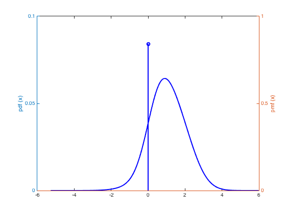
Plot the estimated distribution

figure(1)
plot_GM(EMfin);

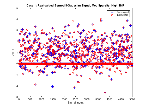
Plot the true and estimated signals

figure(2)
plot(xtrue,'b+');hold on % plot true signal
plot(xhat,'ro'); hold off % plot signal estimate
xlabel('Signal Index'); ylabel('Value')
title('Case 1: Real-valued Bernoulli-Gaussian Signal, Med Sparsity, High SNR')
legend('True signal', 'Est Signal')

Exploiting Prior Signal Knowledge with EM-GM-AMP

Sometimes one has partial knowledge of the signal prior. To exploit this, we can disable the EM learning on one or more parameters.

% Set initial GM parameters at the true values
clear optEM
optEM.active_mean = 1; %Initialize at correct active mean
optEM.active_weights = 1; %Trivial weights since 1-term "mixture"
optEM.active_var = 1; %Initialize correct active variance
optEM.noise_var = wvar; %Initialize at correct noise variance

% Turn off EM learning of all but the sparsity-rate, lambda
optEM.learn_lambda= true;
optEM.learn_mean = false;
optEM.learn_weights = false;
optEM.learn_var = false;
optEM.learn_noisevar = false;

% Run, time, and check performance of EMGMAMP
optEM.heavy_tailed = false; % since operating on a sparse signal
time2 = tic;
[xhat,EMfin] = EMGMAMP(y, Amat,optEM);
time2 = toc(time2)
NMSE_dB2 = 10*log10(norm(xtrue-xhat)^2/norm(xtrue)^2)
sparsity_error_dB = 10*log10(EMfin.lambda/(K/N))

time2 =

    0.5919


NMSE_dB2 =

  -29.9516


sparsity_error_dB =

    0.0030

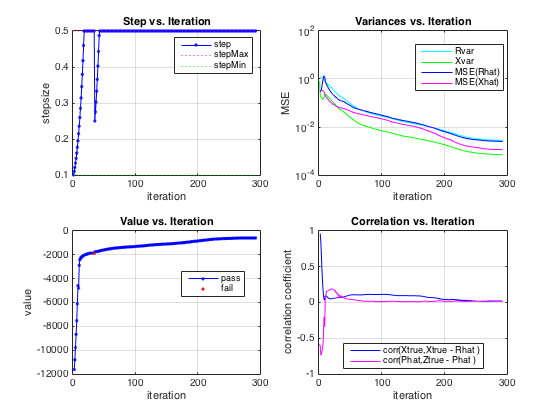
Using the Robust Mode of EM-GM-AMP and Showing the Convergence History

For non-iid measurement matrices, we suggest using EMGMAMP's "robust_gamp" mode. Below we generate a matrix with correlated columns, run EMGMAMP, and show the resulting convergence history. Notice how the damping parameter (i.e., the "stepsize") decreases when the utility function (i.e., the "value") decreases, to help the algorithm converge.

% Generate matrix
clear Params
Params.M = M; Params.N = N; Params.type = 1; Params.realmat = true;
Params.tau = 0.7; % Make columns correlated
Amat = generate_Amat(Params); % Generate the random matrix

% Generate noisy outputs
ztrue = Amat*xtrue; % compute true transform-output vector
wvar = norm(ztrue)^2/M*10^(-SNR/10); % calculate noise level
y = ztrue + sqrt(wvar)*(randn(M,1)); % compute noisy output

% Run, and check performance of EMGMAMP
clear optEM
optEM.robust_gamp = true; % help robustify the convergence
optEM.heavy_tailed = false; % since operating on a sparse signal
[xhat,~,estHist,~,optGAMPfin] = EMGMAMP(y, Amat, optEM);
NMSE_dB4 = 10*log10(norm(xtrue-xhat)^2/norm(xtrue)^2)

% Show convergence history
figure(3)
gampShowHist(estHist,optGAMPfin,xtrue,ztrue);

NMSE_dB4 =

  -24.6896

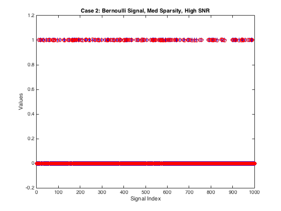
Example 3: Real Bernoulli Signal

Let's see if EM-GM-AMP can learn that the signal takes on only the values {0,1} and exploit its structure for improved reconstruction accuracy.

% Declare dimensions
N = 1000; % signal length
del = 0.4; % measurement-to-signal ratio, M/N
rho = 0.4; % sparsity-to-measurement ratio, K/M
SNR = 30; % SNR (in dB)
M = ceil(del*N); %Find appropriate measurement size
K = floor(rho*M); %Find appropriate sparsity
if K == 0
    K = 1; %Ensure at least one active coefficient.
end

% Generate matrix
clear Params
Params.M = M; Params.N = N; Params.type = 1; Params.realmat = true;
Amat = generate_Amat(Params);

% Generate sparse signal
xtrue = zeros(N,1); % initialize signal vector
xtrue(randperm(N,K)) = 1; %Bernoulli signal

% Generate noisy outputs
ztrue = Amat*xtrue; % compute true transform-output vector
wvar = norm(ztrue)^2/M*10^(-SNR/10); % calculate noise level
y = ztrue + sqrt(wvar)*(randn(M,1)); % compute noisy output

% Run, time, and check performance of EMGMAMP
clear optEM
optEM.heavy_tailed = false; % since operating on a sparse signal
time5 = tic;
[xhat,EMfin] = EMGMAMP(y, Amat, optEM);
%[xhat,EMfin,estHist,~,optGAMPfin] = EMGMAMP(y, Amat, optEM); figure(3); gampShowHist(estHist,optGAMPfin,xtrue,ztrue);
time5 = toc(time5)
NMSE_dB5 = 10*log10(norm(xtrue-xhat)^2/norm(xtrue)^2)

% Plot the true and estimated signals
figure(5)
plot(xtrue,'b+'); hold on
plot(xhat,'ro'); hold off
xlabel('Signal Index'); ylabel('Values')
title('Case 2: Bernoulli Signal, Med Sparsity, High SNR')

time5 =

    0.3639


NMSE_dB5 =

  -53.0791

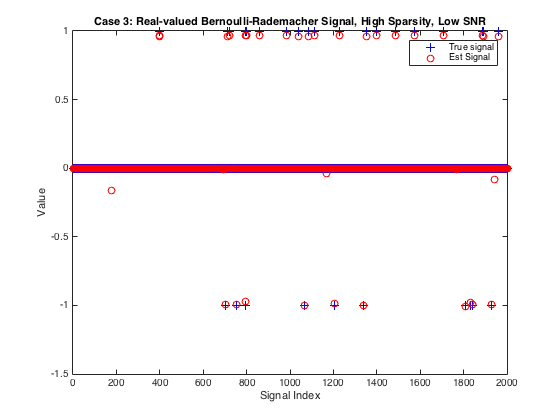
Example 3: Real Bernoulli-Rademacher Signal

Let's see if EM-GM-AMP can learn that the signal takes on only the values {0,-1,+1} and exploit its structure for improved reconstruction accuracy. This time we'll use a lower SNR.

% Declare dimensions
N = 2000; % signal length
del = 0.1; % measurement-to-signal ratio, M/N
rho = 0.15; % sparsity-to-measurement ratio, K/M
SNR = 15; % SNR (in dB)
M = ceil(del*N);
K = floor(rho*M);
if K == 0
    K = 1; %Ensure at least one active coefficient.
end

% Generate matrix
clear Params
Params.M = M; Params.N = N; Params.type = 1; Params.realmat = true;
Amat = generate_Amat(Params);

% Generate sparse signal
xtrue = zeros(N,1);
xtrue(randperm(N,K)) = sign(randn(K,1));

% Generate noisy outputs
ztrue = Amat*xtrue; % compute true transform-output vector
wvar = norm(ztrue)^2/M*10^(-SNR/10); % calculate noise level
y = ztrue + sqrt(wvar)*(randn(M,1)); % compute noisy output

% Run, time, and check performance of EMGMAMP
clear optEM
optEM.heavy_tailed = false; % since operating on a sparse signal
time6 = tic;
xhat = EMGMAMP(y, Amat, optEM);
time6 = toc(time6)
NMSE_dB6 = 10*log10(norm(xtrue-xhat)^2/norm(xtrue)^2) % Report EMGMAMP's NMSE (in dB)

% Plot the true and estimated signals
figure(6)
plot(xtrue,'b+');hold on
plot(xhat,'ro'); hold off
xlabel('Signal Index'); ylabel('Value')
title(sprintf('Case 3: Real-valued Bernoulli-Rademacher Signal, High Sparsity, Low SNR'))
legend('True signal', 'Est Signal')

time6 =

    0.8080


NMSE_dB6 =

  -26.6891

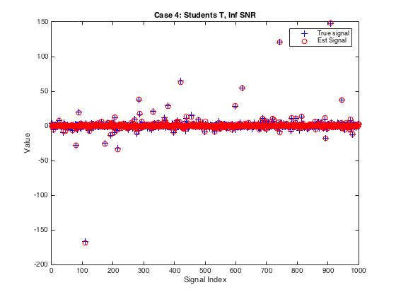
Example 4: Heavy-tailed signal

Lets try EM-GM-AMP on a heavy tailed signal (non-compressible Student's T) with Infinite SNR using a Random Rademacher matrix.

% Declare dimensions
N = 1000; % signal length
del = 0.65; % measurement-to-signal ratio, M/N
SNR = Inf; % SNR (in dB)
M = ceil(del*N);

% Generate matrix
clear Params
Params.M = M; Params.N = N; Params.realmat = true;
Params.type = 2; % specify Rademacher {-1,+1} matrix
Params.realmat = true;
Amat = generate_Amat(Params);

% Generate heavy-tailed, non-sparse signal
xtrue = random('t',1.5,N,1);

% Generate noisy outputs
ztrue = Amat*xtrue; % compute true transform-output vector
wvar = norm(ztrue)^2/M*10^(-SNR/10); % calculate noise level
y = ztrue + sqrt(wvar)*(randn(M,1)); % compute noisy output

% Run, time, and check performance of EMGMAMP
clear optEM
optEM.heavy_tailed = true; % since operating on a heavy-tailed signal
time7 = tic;
xhat = EMGMAMP(y, Amat);
time7 = toc(time7)
NMSE_dB7 = 10*log10(norm(xtrue-xhat)^2/norm(xtrue)^2) % Report EMGMAMP's NMSE (in dB)

% Plot the true and estimated signals
figure(7)
plot(xtrue,'b+'); hold on
plot(xhat,'ro'); hold off
xlabel('Signal Index'); ylabel('Value')
title(sprintf('Case 4: Students T, Inf SNR'))
legend('True signal', 'Est Signal')

time7 =

    1.8272


NMSE_dB7 =

  -18.2786