EM-BG-AMP Algorithm: Usage Examples

Jeremy Vila and Philip Schniter, Nov. 2015

EM-BG-AMP attempts to recover a sparse signal of length N through (possibly) noisy measurements of length M (with perhaps M < N). We model this through the linear system

$\bf{y} = \bf{Ax} + \bf{w}$ .

Please refer to the paper EM-BG-AMP by Jeremy Vila Philip Schniter for a detailed description of the algorithm. This manual will show how to use the EM-BG-AMP MATLAB code and how to intepret the results.

Generating Data
The Standard Way to Invoke EM-BG-AMP
Exploiting Prior Signal Knowledge with EM-BG-AMP
Example 2: Complex Bernoulli-Gaussian Signal
Example 3: Real-valued Bernoulli-Rademacher Signal
Example 4: Real-valued Bernoulli Signal

Generating Data

The following examples will use randomly generated data. First, we create the K-sparse signal, then the M-by-N measurement matrix, and finally the AWGN-corrupted measurements.

clear all
close all

% Check that EMGMAMP.m is on the path
if exist('EMGMAMP.m')~=2
  error('EMGMAMP.m not on the path')
end

% Choose between the new and old versions of EMGMAMP
newEM = true;
EMGMpath = fileparts(which('EMGMAMP')); % current path to EMGM
[GAMPdir,EMGMver] = fileparts(EMGMpath); % GAMPmatlab dir and EMGM version
if newEM
  if strcmp(EMGMver,'EMGMAMP')
    rmpath(EMGMpath)
    addpath([GAMPdir,'/EMGMAMPnew'])
    warning('Changing path from old to new version of EMGMAMP')
  end
else
  if strcmp(EMGMver,'EMGMAMPnew')
    rmpath(EMGMpath)
    addpath([GAMPdir,'/EMGMAMP'])
    warning('Changing path from new to old version of EMGMAMP')
  end
end

% Declare dimensions
N = 1000; % signal length
del = 0.4; % measurement-to-signal ratio, M/N
rho = 0.4; % sparsity-to-measurement ratio, K/M
SNR = 30; % SNR (in dB)
M = ceil(del*N); % measurement length
K = floor(rho*M); % sparsity
if K==0
    K = 1; % ensure at least one active coefficient
end

% Generate matrix
clear Params;
Params.M = M;
Params.N = N;
Params.realmat = true; % specify real-valued matrix
Params.type = 1; % specify i.i.d. Gaussian matrix
Amat = generate_Amat(Params); % generate random matrix

% Generate sparse signal
active_mean = 1; % mean of non-zero components
active_var = 1; % variance of non-zero components
xtrue = zeros(N,1); % initialize signal vector
xtrue(randperm(N,K)) = (sqrt(active_var)*randn(K,1)+active_mean);

% Generate noisy outputs
ztrue = Amat*xtrue; % compute true output vector
wvar = norm(ztrue)^2/M*10^(-SNR/10); % calculate noise level
y = ztrue + sqrt(wvar)*(randn(M,1)); % compute noisy output

The Standard Way to Invoke EM-BG-AMP

Using the EM-BG-AMP algorithm is extremely easy. You simply need the measurements and measurement matrix. The algorithm returns signal estimate, the learned parameters of the assumed Bernoulli-Gaussian prior, as well as the AWGN variance.

% Run, time, and check performance of EMBGAMP
optEM.heavy_tailed = false; % since operating on a sparse signal
time = tic;
[xhat, EMfin] = EMBGAMP(y, Amat, optEM);
time = toc(time)
NMSE_dB = 10*log10(norm(xtrue-xhat)^2/norm(xtrue)^2)
wvar_error_dB = 10*log10(EMfin.noise_var/wvar)
active_mean_error_dB = 10*log10(EMfin.active_mean/active_mean)
active_var_error_dB = 10*log10(EMfin.active_var/active_var)
sparsity_error_dB = 10*log10(EMfin.lambda/(K/N))

time =

    0.4861


NMSE_dB =

  -30.8079


wvar_error_dB =

    0.4500


active_mean_error_dB =

    0.1270


active_var_error_dB =

    0.4844


sparsity_error_dB =

    0.0048

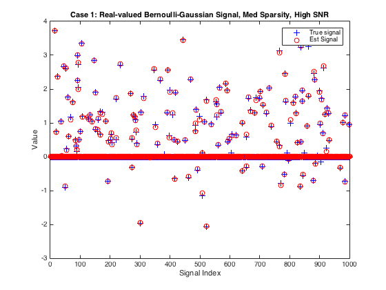
Plot the true and estimated signals

figure(2)
plot(xtrue,'b+');hold on % plot true signal
plot(xhat,'ro'); hold off % plot signal estimate
xlabel('Signal Index'); ylabel('Value')
title('Case 1: Real-valued Bernoulli-Gaussian Signal, Med Sparsity, High SNR')
legend('True signal', 'Est Signal')

Exploiting Prior Signal Knowledge with EM-BG-AMP

Sometimes one has partial knowledge of the signal prior. To exploit this, we can disable the EM learning on one or more parameters.

% Set initial BG parameters at the true values
clear optEM
optEM.active_mean = 1; %Initialize at correct active mean
optEM.active_weights = 1; %Trivial weights since 1-term mixture
optEM.active_var = 1; %Initialize correct active variance
optEM.noise_var = wvar; %Initialize at correct noise variance

% Turn off EM learning of all but the sparsity-rate, lambda
optEM.learn_lambda= true;
optEM.learn_mean = false;
optEM.learn_weights = false;
optEM.learn_var = false;
optEM.learn_noisevar = false;

% Run, time, and check performance of EMBGAMP
optEM.heavy_tailed = false; % since operating on a sparse signal
time2 = tic;
xhat = EMBGAMP(y, Amat,optEM);
time2 = toc(time2)
NMSE_dB2 = 10*log10(norm(xtrue-xhat)^2/norm(xtrue)^2)
sparsity_error_dB = 10*log10(EMfin.lambda/(K/N))

time2 =

    0.0935


NMSE_dB2 =

  -30.9412


sparsity_error_dB =

    0.0048

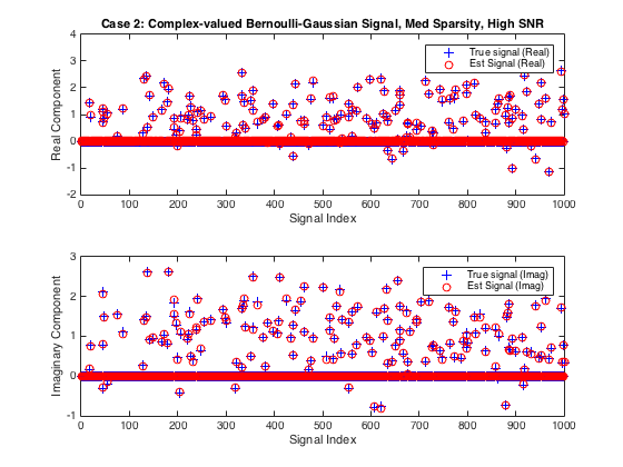
Example 2: Complex Bernoulli-Gaussian Signal

EM-BG-AMP can also handle complex-valued signals and measurements. Let's try it.

% Declare dimensions
N = 1000; % signal length
del = 0.4; % measurement-to-signal ratio, M/N
rho = 0.4; % sparsity-to-measurement ratio, K/M
SNR = 30; % SNR (in dB)
M = ceil(del*N); % measurement length
K = floor(rho*M); % sparsity
if K==0
    K = 1; % ensure at least one active coefficient
end

% Generate matrix
clear Params;
Params.M = M;
Params.N = N;
Params.realmat = false; % specify complex-valued matrix
Params.type = 1; % specify i.i.d. Gaussian matrix
Amat = generate_Amat(Params); % generate random matrix

% Generate sparse signal
active_mean = 1+1i; % mean of non-zero components
active_var = 1; % variance of non-zero components
xtrue = zeros(N,1); % initialize signal vector
xtrue(randperm(N,K)) = (sqrt(active_var/2)*randn(K,2)*[1;1i]+active_mean);

% Generate noisy outputs
ztrue = Amat*xtrue; % compute true output vector
wvar = norm(ztrue)^2/M*10^(-SNR/10); % calculate noise level
y = ztrue + sqrt(wvar/2)*(randn(M,2)*[1;1i]); % compute noisy output

% Run, time, and check performance of EMBGAMP
optEM.heavy_tailed = false; % since operating on a sparse signal
time5 = tic;
[xhat, EMfin] = EMBGAMP(y, Amat, optEM);
time5 = toc(time5)
NMSE_dB5 = 10*log10(norm(xtrue-xhat)^2/norm(xtrue)^2)
wvar_error_dB5 = 10*log10(EMfin.noise_var/wvar)

% Plot the true and estimated signals
figure(2)
subplot(2,1,1)
plot(real(xtrue),'b+'); hold on
plot(real(xhat),'ro'); hold off
xlabel('Signal Index'); ylabel('Real Component')
title('Case 2: Complex-valued Bernoulli-Gaussian Signal, Med Sparsity, High SNR')
legend('True signal (Real)', 'Est Signal (Real)')
subplot(2,1,2)
plot(imag(xtrue),'b+'); hold on
plot(imag(xhat),'ro'); hold off
xlabel('Signal Index'); ylabel('Imaginary Component')
legend('True signal (Imag)', 'Est Signal (Imag)')

time5 =

    0.1741


NMSE_dB5 =

  -32.2383


wvar_error_dB5 =

   -1.2392

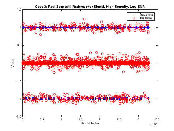
Example 3: Real-valued Bernoulli-Rademacher Signal

Let's see if EM-BG-AMP can learn that the signal takes on only the values {0,1} and exploit its structure for improved reconstruction accuracy. Also, let's use the oversampled DFT operator this time, meaning the measurements are complex but the signal is real-valued.

N = 2^15; % specify power-of-2 value for N
del = 0.1; % measurement-to-signal ratio, M/N
rho = 0.15; % sparsity-to-measurement ratio, K/M
SNR = 15; % SNR (in dB)
M = ceil(del*N); % measurement length
K = floor(rho*M); % sparsity
if K == 0
    K = 1; % ensure at least one active coefficient
end

% Generate matrix
clear Params;
Params.M = M; Params.N = N; Params.realmat = true;
Params.type =3; % specify a DFT operator with random row selection
Amat = generate_Amat(Params);

% Generate sparse signal
xtrue = zeros(N,1);
xtrue(randperm(N,K)) = sign(randn(K,1));

% Generate noisy outputs
ztrue = Amat.mult(xtrue); % compute true output vector
wvar = norm(ztrue)^2/M*10^(-SNR/10); % calculate noise level
y = ztrue + sqrt(wvar/2)*(randn(M,2)*[1;1i]); % compute noisy output

% Run, time, and check performance of EMBGAMP
optEM.heavy_tailed = false; % since operating on a sparse signal
time6 = tic;
[xhat, EMfin] = EMBGAMP(y, Amat, optEM);
time6 = toc(time6)
NMSE_dB6 = 10*log10(norm(xtrue-xhat)^2/norm(xtrue)^2) % Report EMBGAMP's NMSE (in dB)

% Plot the true and estimated signals
figure(6)
plot(xtrue,'b+');hold on
plot(real(xhat),'ro'); hold off
xlabel('Signal Index'); ylabel('Value')
title(sprintf('Case 3: Real Bernoulli-Rademacher Signal, High Sparsity, Low SNR'))
legend('True signal', 'Est Signal')

time6 =

    4.9990


NMSE_dB6 =

  -15.0711

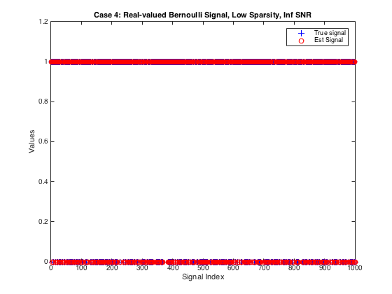
Example 4: Real-valued Bernoulli Signal

Lets try EM-BG-AMP on a Bernoulli signal with Infinite SNR and M=K (sparsity = # measurements) using a Rademacher measurement matrix. Let's also use a tighter stopping tolerance and more iterations to enable a very precise signal estimate.

N = 1000; % specify power-of-2 value for N
del = 0.65; % measurement-to-signal ratio, M/N
rho = 1; % sparsity-to-measurement ratio, K/M
SNR = inf; % SNR (in dB)
M = ceil(del*N); % measurement length
K = floor(rho*M); % sparsity
if K == 0
    K = 1; % ensure at least one active coefficient
end

% Generate matrix
clear Params;
Params.M = M; Params.N = N; Params.realmat = true;
Params.type = 2; % specify Rademacher {-1,+1} matrix
Params.realmat = true;
Amat = generate_Amat(Params);

% Generate sparse signal
xtrue = zeros(N,1); % initialize signal vector
xtrue(randperm(N,K)) = 1; %Bernoulli signal

% Generate noisy outputs
ztrue = Amat*xtrue; % compute true transform-output vector
wvar = norm(ztrue)^2/M*10^(-SNR/10); % calculate noise level
y = ztrue + sqrt(wvar)*(randn(M,1)); % compute noisy output

% Run, time, and check performance of EMBGAMP
clear optEM
optEM.heavy_tailed = false; % since operating on a sparse signal
optGAMP.nit = 500; % increase the number of iterations
optGAMP.tol = 1e-8; % decrease the stopping tolerance
time7 = tic;
xhat = EMBGAMP(y, Amat, optEM, optGAMP);
time7 = toc(time7)
NMSE_dB7 = 10*log10(norm(xtrue-xhat)^2/norm(xtrue)^2)

%Plot signal and the estimates
figure(7)
plot(xtrue,'b+'); hold on
plot(xhat,'ro'); hold off
xlabel('Signal Index'); ylabel('Values')
title(sprintf('Case 4: Real-valued Bernoulli Signal, Low Sparsity, Inf SNR'))
legend('True signal', 'Est Signal')

time7 =

    0.1510


NMSE_dB7 =

 -165.8315